How to Compare Before-and-After Audio With a Spectrogram

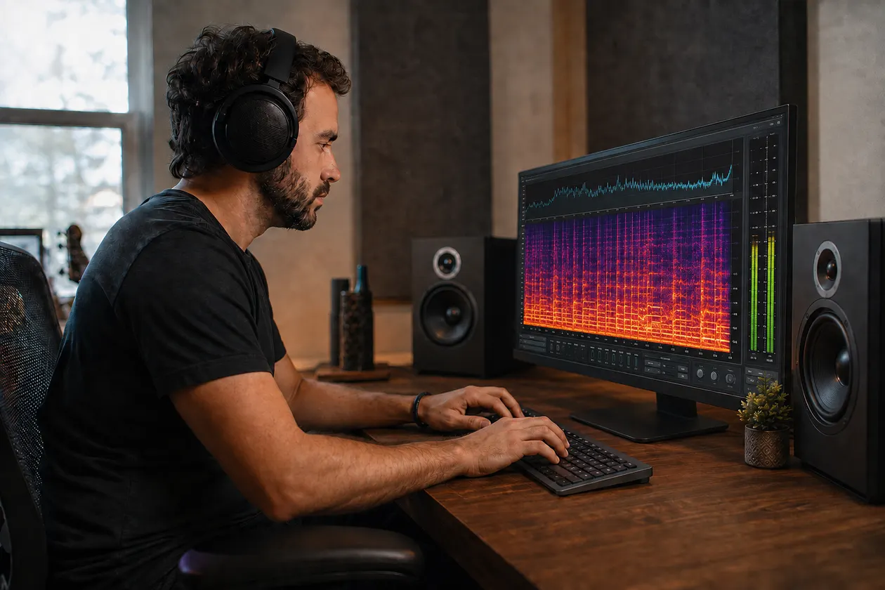
A useful before-and-after spectrogram comparison keeps the source, time selection, analysis settings, display settings, and playback level under control. If any of those change, the picture may look cleaner even though the processing did little, or look busier even though the track sounds better. Match the conditions first, inspect one named sound, and let listening decide whether the change helped.

The practical move is to choose a short passage where you can hear the problem, render both versions with identical settings, and switch between them at similar perceived loudness. A spectrogram can show where displayed energy was reduced or added. It cannot tell you whether that energy was an artifact, a cymbal, vocal air, reverb, or something worth keeping.

I start with the ears because the screen does not know which part of the song matters. I write down the sound and its time before opening a visual tool. That one habit prevents a bright patch from becoming a problem merely because it looks unusual.

Same source and settings

Begin with two files that share one source: the untouched export and one processed candidate. Do not compare an original mix with a later arrangement, a different master, or an extra lossy encode. Those versions contain changes beyond cleanup, so the spectrogram cannot isolate the step you meant to judge.

Align the files to the same sample or obvious transient. A small timing offset makes attacks and consonants appear in different columns. Select the same start and end time, and confirm that both views use the same channel arrangement. A left-channel view is not equivalent to a mono sum, and a stereo pair shown separately is not equivalent to either one.

Most music spectrograms are built with a short-time Fourier transform, or STFT. The signal is divided into overlapping windows, and each window is measured across frequency. SciPy documents the window, hop, sample rate, FFT length, mode, and scaling as explicit parameters. If a tool changes any of them between renders, you are no longer looking at the same measurement setup.

Use one window type and length, one hop or overlap value, one FFT length, and one magnitude or power convention. Match the sample-rate handling too. A longer analysis window can separate steady frequencies more clearly while spreading a quick event across time. A shorter window locates attacks more tightly but groups nearby frequencies into wider bands. Neither setting is inherently more truthful; consistency is what makes the pair comparable.

Then match the display. Audacity’s spectrogram controls include scale, minimum and maximum frequency, gain, range, window, window size, and overlap. Other tools use different names, but the comparison still needs the same frequency scale, vertical limits, decibel reference, color floor, palette, width, height, and interpolation. Turn off per-image automatic contrast when possible. If the software rescales every image to its own brightest point, an unchanged quiet texture can look stronger in the version with the lower peak.

The browser-only spectrogram generator gives you a consistent PNG for a local MP3 or WAV. Use it for both versions when you want a simple repeatable view. Keep the files separate and label them clearly; the tool creates the visualization in browser memory and does not transfer the audio into the cleanup app.

Level matching

Level matching serves two jobs. It makes the listening decision fair, and it stops a broad gain change from dominating the picture. If the processed file is two decibels quieter everywhere, its spectrogram will usually contain darker colors even when the spectral balance is unchanged. Calling that artifact reduction would confuse level with treatment.

Use a loudness meter on the same selected passage if one is available. ITU-R BS.1770 defines algorithms for measuring programme loudness and true peak, and EBU R 128 builds a loudness-normalization recommendation on that foundation. For a short production comparison, the reading is a common starting point rather than a pass/fail target. You still need to hear whether the two versions arrive at roughly the same perceived level.

Lower the louder version with a plain gain control. Do not add a limiter, compressor, EQ, or normalization process that changes the material you are evaluating. Switch the same phrase several times and adjust in small steps until neither version announces itself through a general jump in weight or presence.

Peak matching alone is weak evidence. Two files can hit the same highest peak while one stays dense for most of the passage and sounds louder. Whole-song integrated loudness can also hide a local mismatch in the ten seconds you are testing. Measure the chosen excerpt, then check it by ear.

Keep the monitor or headphone volume unchanged during the switch. Use a comfortable level, then repeat quietly. Loud playback can make upper-frequency detail feel more impressive or more irritating, and tired ears start approving darkness simply because it is easier to tolerate.

Once the audible levels match, use the same display reference for both spectrograms. If the viewer supports a fixed full-scale decibel reference, keep it fixed. Do not normalize each image independently after matching the files, because that erases the very level relationship you just controlled.

Visible reductions and additions

Read a spectrogram as a map of displayed energy over time and frequency. A reduction means that a region contains less measured energy under the matched settings. An addition means that it contains more. Those are observations, not quality judgments.

Start with the sound you named. If a thin metallic layer follows a held vocal between 4 and 8 kHz, mark the corresponding time and frequency area in both images. Ask whether the after version shows a repeatable reduction there. Then listen to the held vocal. If the metallic edge recedes while the word remains clear and open, the visual and audible evidence point in the same useful direction.

Now check neighboring material. A broad darkening across the upper range may include less shimmer, but it may also include shorter cymbal tails, duller consonants, and less room detail. The picture cannot separate wanted and unwanted energy for you. A narrow visual change is not automatically safe either; it might remove part of a note or emphasize the edge around it.

Added energy deserves the same care. Cleanup can expose a bass note that was masked, restore perceived air, change peak control, or alter the balance between components. A brighter region might support clarity, or it might be new harshness. Listen at the exact time, identify the musical source, and compare the complete phrase before deciding.

Do not judge the pair by total brightness. Color maps translate values into colors, and small range changes can make one image look much more dramatic. Use the axes and legend. If the tool offers a frequency-difference panel, treat reduced and added zones as directions for listening, not a score that the after version should maximize.

A good note is modest and auditable: “Under matched settings, energy around this held vowel is lower, and the glassy layer is less distracting at matched playback level.” A weak note says, “The after image is darker, so it is fixed.” The first statement names the place, sound, and listening condition. The second rewards the appearance of cleanup.

Listening order

Use a fixed order so your expectation does not lead the result. First listen to the original without watching the screen. Name one symptom in ordinary language and mark its time. Next listen to the processed version at the matched level. Only then compare the spectrograms and return to the exact passage they highlight.

Switch in short loops of roughly two to five seconds when you are identifying a fine texture. Follow one attribute per pass: metallic edge, hiss between phrases, vocal diction, cymbal decay, depth, or punch. After the short loop, play the complete phrase and the transition into the next section. A treatment that wins on one syllable can still make the musical line feel smaller.

I usually check the busiest chorus first. That is where upper-frequency textures are easier to hear, and where broad processing can remove the most wanted material at once. I pair that chorus with one exposed verse or intro, because the quiet passage reveals residue while the chorus reveals collateral damage.

Try the sequence original, after, original. Returning to the source catches the tendency to adapt to the last thing heard. When the difference is close, hide the filenames or ask someone else to switch them. You do not need a formal listening laboratory, but you do need a way to notice when you prefer the version you expected to prefer.

Use the image after each audible decision, not continuously. Looking at a darkened band while switching can make you listen for an improvement that may not be there. Once you have chosen by ear, inspect whether the visual change lands at the same time and frequency. If it does not, recheck alignment, settings, and your description before adding more processing.

If the artifact remains, make one small adjustment on a new copy and repeat the same passage. The broader artifact-removal workflow helps you decide whether the next step is a restrained EQ move, denoise, track-aware cleanup, stem work, regeneration, mastering, or no further change.

Limits of visual comparison

A spectrogram complements listening. It does not issue an automatic diagnosis. Bright high-frequency energy can be a cymbal, consonant, synth harmonic, noise, reverb, or an unwanted synthetic texture. A dark region can mean silence, a low display floor, a frequency limit, or musical content below the chosen range.

The image also cannot establish how a closed generator works internally or where a track came from. Similar patterns can follow arrangement, performance, effects, encoding, resampling, level changes, and rendering choices. Keep provenance questions separate from sound-quality decisions.

Do not process toward a prettier picture. An after view with less upper energy may correspond to a duller vocal. A smoother tail may come from removing ambience that gave the song depth. A stronger low band may be useful body or unwanted buildup. The only reliable question is whether the named sound improved without unacceptable musical cost.

There are source problems that broad cleanup cannot reverse. Heavy clipping, missing detail, broken timing, a wrong note, a poor performance, and an unwanted arrangement call for different work. A finished stereo mix also limits how independently you can change the vocal, cymbals, bass, and effects. The cleanup-versus-mastering guide explains why repair, balance, loudness, and final polish should remain separate decisions.

I built Sunofix for the stage where the song already works but the exported mix still has a broad synthetic edge. It can create a cleaner WAV and give you before-and-after playback, spectrogram comparison, and frequency diagnostics. It cannot restore missing source detail, rewrite lyrics or melody, repair an arrangement or performance, replace stem-level mixing, complete mastering, or guarantee approval from a distributor.

Compare before and after fairly with the untouched export nearby. Keep the result only if the audible benefit survives level matching and the song retains its clarity, movement, and emotional shape.

Decision checklist

Use this short record for each candidate:

1. Confirm that before and after come from the same source and differ only by the treatment under review.
2. Align the same passage and channel choice in both versions.
3. Match window, hop or overlap, FFT length, scaling, frequency range, decibel reference, palette, and image dimensions.
4. Disable automatic per-image contrast, or retain both legends if it cannot be disabled.
5. Match the selected passage by perceived loudness using a meter as the starting point and gain only for correction.
6. Write one audible target with a timestamp before looking at the images.
7. Switch a short loop and follow that target alone.
8. Mark visible reductions and additions at the same time and frequency, then listen again.
9. Check wanted neighbors: diction, cymbal decay, transients, bass stability, width, depth, and ambience.
10. Play the full phrase, the busiest chorus, and one exposed section.
11. Repeat quietly and on a second familiar playback system if the decision matters.
12. Keep the lightest pass that makes the named problem less distracting without making the song darker, flatter, narrower, quieter, or less alive.

Record the passage, gain offset, settings, audible improvement, and audible cost. If you cannot describe the improvement without referring to the picture, return to the original and listen again. If the after version needs a level advantage or aggressive display scaling to look convincing, it has not earned the decision.

Stop when the target is less distracting and the parts you wanted to preserve still work. A small remaining artifact can be a better trade than a lifeless cleanup. The spectrogram has done its job when it leads you back to the right seconds, helps you repeat the comparison, and then gets out of the way of the song.